Levenberg-Marquardt algorithm with numeric Jacobians
1. Examples
If you prefer directly jumping to example code, see:
2.Introduction
This page first describes the Levenberg-Marquardt optimization algorithm, then shows how to use its implementation within the mrpt-math C++ library. All the source code discussed here, the implementation of the algorithm itself, and the examples, are available for download within the MRPT packages.
The following notation and algorithm have been extracted from the report [2]
3. Algorithm description
The Levenberg-Marquardt (LM) method consists on an iterative least-square minimization of a cost function based on a modification of the Gauss-Newton method. Let’s state the problem formally before defining the algorithm. We will assume that derivatives of the cost functions are not available in closed form, so they will be approximated by finite-difference approximation Finite-difference approximation.
Let \(\mathbf{x} \in \mathcal{R}^n\) be the parameter vector to be optimized. We want to find the optimal \(\mathbf{x}^\star\) that minimizes the scalar error function \(F(\cdot)\) :
with:
The function \(\mathbf{f}: \mathcal{R}^n \to \mathcal{R}^m\) may sometimes include a comparison to some reference, or observed, data. A very simple, linear example would be \(\mathbf{f}(\mathbf{x}) = \mathbf{b} - \mathbf{A}\mathbf{x}\). However in the following we assume \(\mathbf{f}(\cdot)\) can have any form:
We define the Jacobian of the error functions as the \(m \times n\) matrix:
The Hessian of the error function is the \(n \times n\) matrix of second order derivatives (\(n\) being the length of the parameter vector), and it’s approximated by:
If we do not have closed form expressions for the derivatives needed for the Jacobian, we can estimate them from finite differences using some increments for each individual variable \(\Delta x_j\) :
Then, the LM method minimizes the following linear approximation of the actual error function:
where the gradient \(\mathbf{g}(x)\) is given by \(\mathbf{J}(x)^T \mathbf{f}(x)\).
Now, denote as \(\mathbf{x}^\star_{t}\) for \(t=0,1,2,...\) the sequence of iterative approximations to the optimal set of parameters \(\mathbf{x}^\star\). The first initial guess \(\mathbf{x}^\star_0\) must be provided by the user. Then, each iteration of the LM method performs:
where each step is obtained from:
The damping factor \(\lambda\) is adapted dynamically according to a heuristic rule, as shown in the next list of the whole algorithm. Basically, it iterates until a maximum number of iterations is reached or the change in the parameter vector is very small.
4. C++ Implementation
The LM algorithm is implemented in the C++ template class mrpt::math::CLevenbergMarquardtTempl<T>, and there is an example in MRPT/samples/optimize-lm, which is described next.
The type mrpt::math::CLevenbergMarquard is actually a shortcut for the template instantiation mrpt::math::CLevenbergMarquardtTempl<double>.
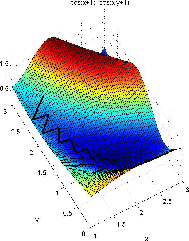
The image below represents the resulting path from the initial guess to the minimum for this example. The displayed equation is the one-dimensional error (cost) function, \(\mathbf{f}(\mathbf{x})\) :
